

SITCOMTN-128
Unrecognized Blends in LSSTComCam Data Preview 1 ECDFS#
Abstract
Unrecognized blends are a class of blended objects where two (or more) objects are so close on the sky that they are mistakenly identified as a single object. These objects can cause a variety of issues for science and simple validation. We can identify such objects by using higher resolution imaging from a space based telescope that will not be affected by ground based seeing and then label detected objects as isolated, recognized blends, or unrecognized blends. We find that for objects with 23 < i < 24.5, 18% of objects are unrecognized blends.
DOI: https://doi.org/10.71929/rubin/2570850
Data#
The Extended Chandra Deep Field-South (ECDFS), or also known as GOODS-South, is an extension to the original Chandra Deep Field-South which was originally observed in X-Rays but has since been observed across many bands.
The Vera Rubin Observatory’s LSST Commissioning Camera (LSSTComCam) [SLAC National Accelerator Laboratory and NSF-DOE Vera C. Rubin Observatory, 2024] observed this patch of sky with over 1000 visits in total, 250 being in the \(i\)-band alone, similar to 10-year depth [Guy et al., 2025].
This data was then processed several times through the Rubin pipelines enabling rapid improvements to the entire system.
Unrecognized blends allow us to understand some of the inherent failure modes of object detection when objects are too close on the sky to be differentiated.
We use the /repo/dp1 repo and LSSTComCam/runs/DRP/DP1/v29_0_0/DM-50260 collection for LSSTComCam data along with HST CANDELS data [Grogin et al., 2011, Guo et al., 2013, Koekemoer et al., 2011].
The DP1 Object catalog [NSF-DOE Vera C Rubin Observatory, 2025, NSF-DOE Vera C. Rubin Observatory, 2025] includes a deblending algorithm which means with accurate detection it is able to parse isolated and “recognized blends.”
Deblending produces “children” objects from a “parent object”, both of which are in the catalog and needs to be pruned in order to remove duplicates.
We apply the general detect_isPrimary flag which removes the parent objects (if child object exist) from the catalog along with removing any sky objects and that the object is from the inner part of both a tract and a patch.
We will use the terms “extended object” (defined by refExtendedness == 1) and “observed galaxy” interchangibly.
We place two cuts on the HST catalog, that the F814W magnitude be brighter than tunable value which we call the space magnitude (\(m_s\)) and that FLAG == 0 which removes only 318 objects.
Details on the HST FLAG parameter can be found here.
The overlap between the two catalogs can be seen in Fig. 1 and the magnitude distribution (\(i\) for LSSTComCam and F814W for HST) in Fig. 7.
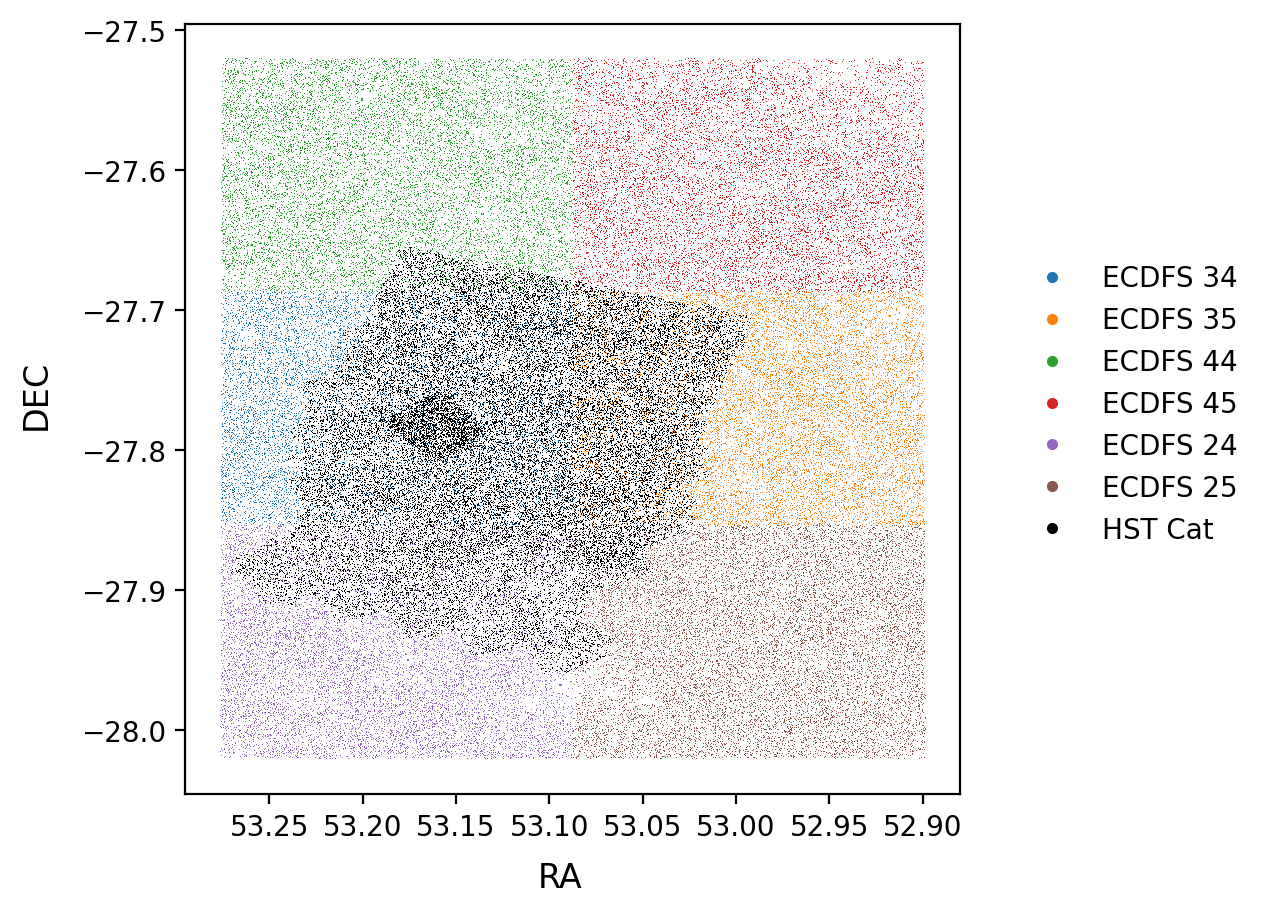
Fig. 1 Footprint of the two surveys. HST is shown in black and DP1 data is shown in the non-black points. Each non-black color refers to a different patch in the ECDFS DP1 data.#
Matching#
Ground and space catalogs in hand, we can start to label objects in the ground catalog as isolated objects (pure), recognized blends, or unrecognized blends by matching between the two catalogs. The general idea will be to generate a list of candidate unrecognized blends and then refine that list, e.g. by removing any unrecognized blends that are unlikely to be contaminated (a 23-mag blended with a 27 mag), as well as removing residual pure objects and recognized blends.
Seemingly the simplest way to match between the two catalogs would be to use pure spatial information, RA and DEC.
Querying the ground and space catalogs within some search_radius (which we choose to be the same for both catalogs) and then comparing the counts which can be done quickly using a k-d tree datastructure like the one implemented in scipy [Virtanen et al., 2020] as scipy.spatial.kdtree.
This can work well for pure objects but introduces a dependence on the search_radius parameter.
Moreover, purely spatial matching can mistanekly label recognized blends as unrecognized blends.
However, it is a common matcher so the results are included below but elect to pursue a more involved ellipse matcher outlined in [Liang et al., 2025].
The ellipse matcher uses the position (RA, DEC) and shape parameters (A, B, \(\Theta\)) to model objects in both catalogs as ellipses and then require that there be overlap between the ground ellipse and space ellipse in order for an object to be labelled as a blend.
If there are multiple space ellipses overlapping with the same ground ellipse, that object is an unrecognized blend.
For DP1, the shape parameters come from shape_xx, shape_xy, and shape_yy that can be converted to A, B, and \(\Theta\) while the HST catalog includes these values as measured from Source Extractor.
Note that a pixel-to-arcsecond factor must be used to make sure that the two catalogs have meaningfully consistent units when we make comparisons.
The center of each object, measured by RA and DEC, with the above parameters, A, B, and \(\Theta\), can be used to write an analytic expression for the ellipse:
Parameterizing this way allows us to efficiently determine if there is overlap with other ellipses.
Note that the typical ellipse parameters of the semimajor axis, A, and semi-minor axis, B, do not correspond to the coefficients of this polynomial written as \(\hat{A}\), \(\hat{B}\).
On average, the product \(\sqrt{A \times B} \approx\) the half-light radius so we scale both parameters by a candidate_boost_factor which we will set to 2 unless otherwise specified.
This factor comes from visual inspection that twice the half-light radius is better able to recreate the object’s profile.
For each ground object, we query for objects within 5’’ of the original ground object in both the ground and space catalog and determine if there is any overlap in either catalog.
We query the ground catalog to account for recognized blends.
If there are more space objects (\(\hat{N_s}\)) than ground objects (\(\hat{N_g}\)), the object is a candidate unrecognized blend.
If there are equal amounts then the object is either pure (\(\hat{N_s} = \hat{N_g} = 1\)) or recognized blend (\(\hat{N_s} = \hat{N_g} > 1\)).
In the case of missing space data or spurious detections (\(\hat{N_g} > \hat{N_s}\)), the object is ignored for subsequent analysis.
Once we have a set of candidate blends, we apply cuts based on the space magnitude to isolate to the most problematic unrecognized blends. Against HST we focus on the F814W band but this can be applied to any band observed by a space instrument. We require that:
The space objects are brighter than a limit \(m_s\). This removes faint objects that are unlikely to be detected by our instrument and reduce computational overhead.
The difference between the faintest and brightest space match, \(m_{bright} - m_{faint} = \Delta_m\), is less than a difference limit \(m_\Delta\).
The first cut can be understood as requiring completeness in the space catalog with the second restricting our search to blends that are likely to have an impact on measured properties such as flux and shape. Once applying the cuts on the space catalog we recount the number of objects in the sets and promote any surviving candidate unrecognized blends to unrecognized blends.
In summary, for each ground detection (original object)
Querying a radius \(r\) around the ground detection RA and DEC in the ground catalog gives \(\hat{N_g}\) ground objects.
Querying a radius \(r\) around the ground detection RA and DEC in the space catalog gives \(\hat{N_s}\) space objects.
Convert each of the \(\hat{N_g}\) and \(\hat{N_s}\) objects into ellipses.
Of the \(\hat{N_g}\) ground objects, only \(N_g\) have overlap with the original object.
Of the \(\hat{N_s}\) space objects, only \(N_s\) have overlap with the original object.
If \(N_s > N_g\) we have a candidate unrecognized blend.
If \(N_s \leq N_g\) we have a recognized blend or a spurious detection.
When using the the spatial matcher, we skip steps 3 to 5 for each ground object and use a smaller search radius to generate a list of candidate blends.
Each method is then refined using the same magnitude requirements on the space matches:
\(m_{F814} < m_s\).
- \(m_{bright} - m_{faint} = \Delta_{F814} < m_\Delta\).
We use this cut to remove space matches that are contributing a negligible amount of flux compare to the brightest space match.
In total, we use two matching algorithms, ellipse and spatial to generate a list of candidate blends and then refine using the same magnitude requirements.
Unrecognized Blends#
Using the matching schemes detailed above we can label isolated objects (pure), recognized blends and unrecognized blends in the ground catalog.
Unless otherwise specified, we set candidate_boost_factor = 2, \(m_s = 26.5\), and \(m_\Delta = 2\).
Due to setting \(m_\Delta = 2\), even though the LSSTComCam \(i\)-mag distribution peaks at 25, we are only able to confidently label blends up to \(m_g = 24.5\) because the HST catalog is complete only up to \(m_{F814W} = 26.5\) as shown in Fig. 7.
When relevant, the simpler KDTree method will also be presented showing results using search_radius = candidate_boost_factor.
Magnitude Dependence#
We expect that blending will increase at the higher magnitudes as fainter objects are both more abundant (sharp increase in the number density) and harder to uniformly detect. The fraction of unrecognized blends as a function of the observed i-mag is shown in Fig. 2 with a comparison between the two methods included. Restricting to only extended objects – observed galaxies – produces minimal change in the distribution of unrecognized blends.
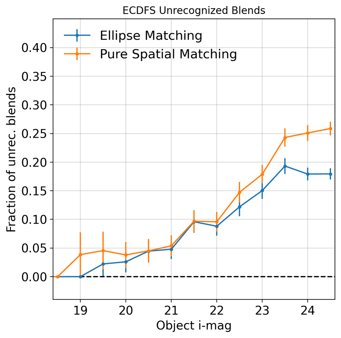
Fig. 2 Fraction of unrecognized blends as a function of observed i-mag. Ellipse matching results are shown in blue and pure spatial results using blend entropy in orange. The two show a similar trend with spatial matching overestimating the number of blends.#
In comparison to the Roman-Rubin simulations [Troxel et al., 2023], we see find similar levels of blending when using purely spatial matching but slightly lower with the ellipse matching.
Shape Parameters#
Accurate shape measurements is necessary for weak lensing studies and it is expected that unrecognized blends will impact any shape estimates. This exact relationship was studied in some of the first work on unrecognized blends in [Dawson et al., 2015] focusing on Subaru data. We repeat that analysis on LSSTComCam data and restrict to galaxies for this section.
Using the second moments of extedned objects, \(Q_{ij}\), we combine into KSB [Kaiser et al., 1995] ellipticity components \(e_1\) and \(e_2\) defined as
The distribution of unrecognized blends as a function of \(e_1\) and \(e_2\) can be found in Fig. 3 and a comparison between the distributions of those components for unrecognized and isolated objects in Fig. 4.
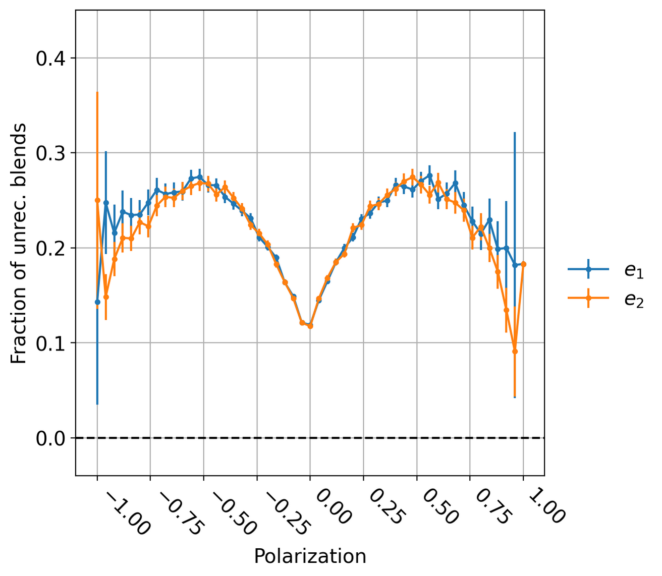
Fig. 3 Fraction of unrecognized blend as a function of ellipse polarization on observed galaxies.#
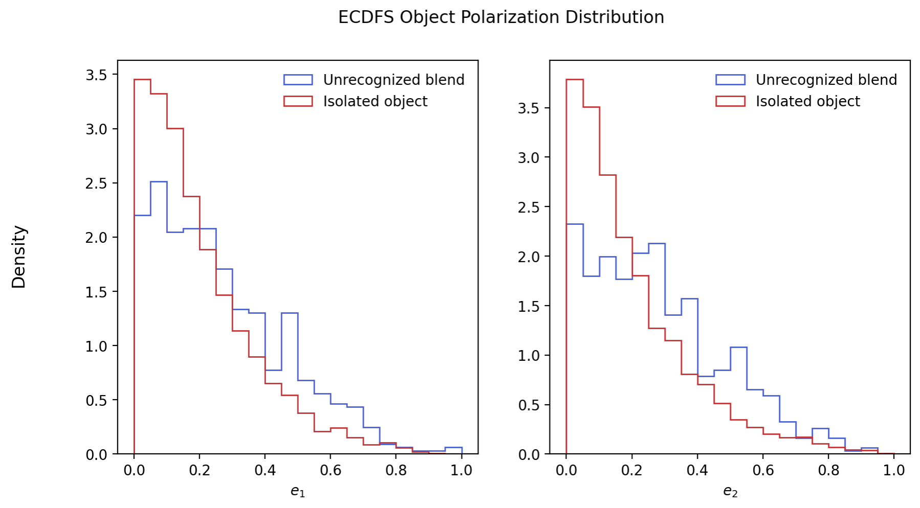
Fig. 4 Normalized distribution of \(e_1\) and \(e_2\) for unrecognized blends (blue) and isolated objects(red). Note that the same same overall pattern between \(|e|\) and \(e_i\) exists persists and there is a negligible difference in shape for the two components.#
Given that there is little to no difference among the shape parameters, \(e_1\) and \(e_2\), this gives good confidence that the pixel grid is not impacting shape measurements and unrecognized blends in strange ways. We also measure the total ellipticity, \(|e|\), as defined in [Dawson et al., 2015]
The distribution of \(|e|\) for isolated and unrecognized blends is shown in Fig. 5.
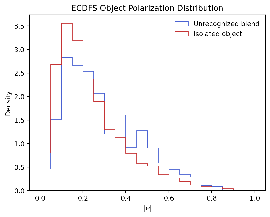
Fig. 5 Normalized distribution of e for unrecognized blends (blue) and isolated objects (red). The longer tail for unrecognized blends is expected as the non-zero angular separation between blends causes a larger ellipticity.#
The offset in \(|e|\) matches the winged structure as unrecognized blends likely have a non-zero angular separation which causes a larger total ellipticity.
Local Density#
Finally, we know clusters and other dense fields (like the deep fields) are expected to be extremely blended which motivates looking into how local density affects unrecognized blend fraction.
To estimate the local density, \(\sum(r_i)\), we use a weighted sum of distances to the \(k\) nearest neighbors following [Darvish et al., 2015].
Where \(d_{ij}\) is the distance between object \(i\) and \(j\) and \(k\) is the number of neighbors which we set to 5. We look at both the ground and space based catalog and calculate two independent densities.
The relationship of unrecognized blends and local density are shown in Fig. 6.
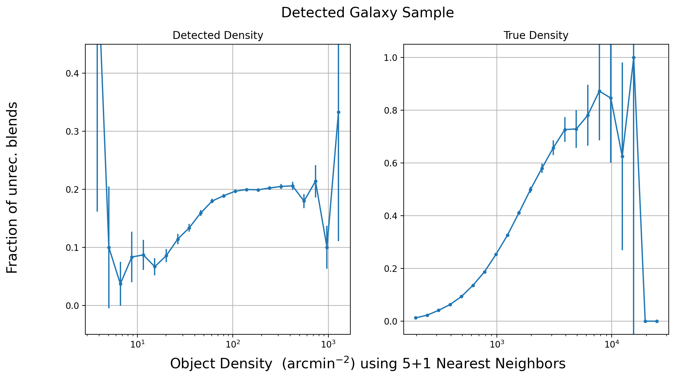
Fig. 6 Fraction of unrecognized blend as a function of LSSTComCam object density (blue) and HST object density (orange).#
As expected, the fraction of unrecognized blends monotonically increases with HST density; however, rather unexpectedly, we see that the blending rate decreases with the ground based LSSTComCam density. We conclude that the LSSTComCam measured object density is not a good predictor of the incidence of blends.
Conclusion#
We have outlined a matching scheme that allows for robustly classifying objects as isolated, recognized blends and unrecognized blends. Using the ellipse matching method, we investigate the occurance of unrecognized blends in the LSSTComCam ECDFS data and how it varies with several properties like i-mag and local density. Comparing to simulations like the Roman-Rubin simulation, we find similar rates of unrecognized blends versus i-magnitude when using purely spatial matching but not ellipse matching. In total, unrecognized blends in LSSTComCam is at the expected levels and not suffering from pipeline issues.
Acknowledgements#
AvdL is supported by the U.S. Department of Energy under award DE-SC0018053. AvdL and PA are supported by the U.S. Department of Energy under awards DE-SC0025309 and DE-SC0023387. PA was also supported in part by the Stony Brook Lourie Fellowship.
This work is based on observations taken by the CANDELS Multi-Cycle Treasury Program with the NASA/ESA HST, which is operated by the Association of Universities for Research in Astronomy, Inc., under NASA contract NAS5-26555.
References#
Behnam Darvish, Bahram Mobasher, David Sobral, Nicholas Scoville, and Miguel Aragon-Calvo. A comparative study of density field estimation for galaxies: new insights into the evolution of galaxies with environment in cosmos out toz∼ 3. The Astrophysical Journal, 805(2):121, May 2015. URL: http://dx.doi.org/10.1088/0004-637X/805/2/121, doi:10.1088/0004-637x/805/2/121.
William A. Dawson, Michael D. Schneider, J. Anthony Tyson, and M. James Jee. The ellipticity distribution of ambiguously blended objects. The Astrophysical Journal, 816(1):11, December 2015. URL: http://dx.doi.org/10.3847/0004-637X/816/1/11, doi:10.3847/0004-637x/816/1/11.
Leanne P. Guy, Keith Bechtol, Eric Bellm, Bob Blum, Gregory P. Dubois-Felsmann, Melissa L. Graham, Željko Ivezić, Robert H. Lupton, Phil Marshall, Colin T. Slater, and Michael Strauss. Rubin Observatory Plans for an Early Science Program. Technical Note RTN-011, Vera C. Rubin Observatory, May 2025. URL: https://rtn-011.lsst.io/, doi:{10.5281/zenodo.5683848}.
Shuang Liang, Prakruth Adari, and Anja von der Linden. Catalog-based detection of unrecognized blends in deep optical ground based catalogs. 2025. URL: https://arxiv.org/abs/2503.16680, arXiv:2503.16680.
Pauli Virtanen, Ralf Gommers, Travis E. Oliphant, Matt Haberland, Tyler Reddy, David Cournapeau, Evgeni Burovski, Pearu Peterson, Warren Weckesser, Jonathan Bright, Stéfan J. van der Walt, Matthew Brett, Joshua Wilson, K. Jarrod Millman, Nikolay Mayorov, Andrew R. J. Nelson, Eric Jones, Robert Kern, Eric Larson, C J Carey, İlhan Polat, Yu Feng, Eric W. Moore, Jake VanderPlas, Denis Laxalde, Josef Perktold, Robert Cimrman, Ian Henriksen, E. A. Quintero, Charles R. Harris, Anne M. Archibald, Antônio H. Ribeiro, Fabian Pedregosa, Paul van Mulbregt, and SciPy 1.0 Contributors. SciPy 1.0: Fundamental Algorithms for Scientific Computing in Python. Nature Methods, 17:261–272, 2020. doi:10.1038/s41592-019-0686-2.
Norman A. Grogin, Dale D. Kocevski, S. M. Faber, Henry C. Ferguson, Anton M. Koekemoer, Adam G. Riess, Viviana Acquaviva, David M. Alexander, Omar Almaini, Matthew L. N. Ashby, Marco Barden, Eric F. Bell, Frédéric Bournaud, Thomas M. Brown, Karina I. Caputi, Stefano Casertano, Paolo Cassata, Marco Castellano, Peter Challis, Ranga-Ram Chary, Edmond Cheung, Michele Cirasuolo, Christopher J. Conselice, Asantha Roshan Cooray, Darren J. Croton, Emanuele Daddi, Tomas Dahlen, Romeel Davé, Duília F. de Mello, Avishai Dekel, Mark Dickinson, Timothy Dolch, Jennifer L. Donley, James S. Dunlop, Aaron A. Dutton, David Elbaz, Giovanni G. Fazio, Alexei V. Filippenko, Steven L. Finkelstein, Adriano Fontana, Jonathan P. Gardner, Peter M. Garnavich, Eric Gawiser, Mauro Giavalisco, Andrea Grazian, Yicheng Guo, Nimish P. Hathi, Boris Häussler, Philip F. Hopkins, Jia-Sheng Huang, Kuang-Han Huang, Saurabh W. Jha, Jeyhan S. Kartaltepe, Robert P. Kirshner, David C. Koo, Kamson Lai, Kyoung-Soo Lee, Weidong Li, Jennifer M. Lotz, Ray A. Lucas, Piero Madau, Patrick J. McCarthy, Elizabeth J. McGrath, Daniel H. McIntosh, Ross J. McLure, Bahram Mobasher, Leonidas A. Moustakas, Mark Mozena, Kirpal Nandra, Jeffrey A. Newman, Sami-Matias Niemi, Kai G. Noeske, Casey J. Papovich, Laura Pentericci, Alexandra Pope, Joel R. Primack, Abhijith Rajan, Swara Ravindranath, Naveen A. Reddy, Alvio Renzini, Hans-Walter Rix, Aday R. Robaina, Steven A. Rodney, David J. Rosario, Piero Rosati, Sara Salimbeni, Claudia Scarlata, Brian Siana, Luc Simard, Joseph Smidt, Rachel S. Somerville, Hyron Spinrad, Amber N. Straughn, Louis-Gregory Strolger, Olivia Telford, Harry I. Teplitz, Jonathan R. Trump, Arjen van der Wel, Carolin Villforth, Risa H. Wechsler, Benjamin J. Weiner, Tommy Wiklind, Vivienne Wild, Grant Wilson, Stijn Wuyts, Hao-Jing Yan, and Min S. Yun. CANDELS: The Cosmic Assembly Near-infrared Deep Extragalactic Legacy Survey. \apjs , 197(2):35, December 2011. arXiv:1105.3753, doi:10.1088/0067-0049/197/2/35.
Yicheng Guo, Henry C. Ferguson, Mauro Giavalisco, Guillermo Barro, S. P. Willner, Matthew L. N. Ashby, Tomas Dahlen, Jennifer L. Donley, Sandra M. Faber, Adriano Fontana, Audrey Galametz, Andrea Grazian, Kuang-Han Huang, Dale D. Kocevski, Anton M. Koekemoer, David C. Koo, Elizabeth J. McGrath, Michael Peth, Mara Salvato, Stijn Wuyts, Marco Castellano, Asantha R. Cooray, Mark E. Dickinson, James S. Dunlop, G. G. Fazio, Jonathan P. Gardner, Eric Gawiser, Norman A. Grogin, Nimish P. Hathi, Li-Ting Hsu, Kyoung-Soo Lee, Ray A. Lucas, Bahram Mobasher, Kirpal Nandra, Jeffery A. Newman, and Arjen van der Wel. CANDELS Multi-wavelength Catalogs: Source Detection and Photometry in the GOODS-South Field. \apjs , 207(2):24, August 2013. arXiv:1308.4405, doi:10.1088/0067-0049/207/2/24.
Nick Kaiser, Gordon Squires, and Tom Broadhurst. A Method for Weak Lensing Observations. \apj , 449:460, August 1995. arXiv:astro-ph/9411005, doi:10.1086/176071.
Anton M. Koekemoer, S. M. Faber, Henry C. Ferguson, Norman A. Grogin, Dale D. Kocevski, David C. Koo, Kamson Lai, Jennifer M. Lotz, Ray A. Lucas, Elizabeth J. McGrath, Sara Ogaz, Abhijith Rajan, Adam G. Riess, Steve A. Rodney, Louis Strolger, Stefano Casertano, Marco Castellano, Tomas Dahlen, Mark Dickinson, Timothy Dolch, Adriano Fontana, Mauro Giavalisco, Andrea Grazian, Yicheng Guo, Nimish P. Hathi, Kuang-Han Huang, Arjen van der Wel, Hao-Jing Yan, Viviana Acquaviva, David M. Alexander, Omar Almaini, Matthew L. N. Ashby, Marco Barden, Eric F. Bell, Frédéric Bournaud, Thomas M. Brown, Karina I. Caputi, Paolo Cassata, Peter J. Challis, Ranga-Ram Chary, Edmond Cheung, Michele Cirasuolo, Christopher J. Conselice, Asantha Roshan Cooray, Darren J. Croton, Emanuele Daddi, Romeel Davé, Duilia F. de Mello, Loic de Ravel, Avishai Dekel, Jennifer L. Donley, James S. Dunlop, Aaron A. Dutton, David Elbaz, Giovanni G. Fazio, Alexei V. Filippenko, Steven L. Finkelstein, Chris Frazer, Jonathan P. Gardner, Peter M. Garnavich, Eric Gawiser, Ruth Gruetzbauch, Will G. Hartley, Boris Häussler, Jessica Herrington, Philip F. Hopkins, Jia-Sheng Huang, Saurabh W. Jha, Andrew Johnson, Jeyhan S. Kartaltepe, Ali A. Khostovan, Robert P. Kirshner, Caterina Lani, Kyoung-Soo Lee, Weidong Li, Piero Madau, Patrick J. McCarthy, Daniel H. McIntosh, Ross J. McLure, Conor McPartland, Bahram Mobasher, Heidi Moreira, Alice Mortlock, Leonidas A. Moustakas, Mark Mozena, Kirpal Nandra, Jeffrey A. Newman, Jennifer L. Nielsen, Sami Niemi, Kai G. Noeske, Casey J. Papovich, Laura Pentericci, Alexandra Pope, Joel R. Primack, Swara Ravindranath, Naveen A. Reddy, Alvio Renzini, Hans-Walter Rix, Aday R. Robaina, David J. Rosario, Piero Rosati, Sara Salimbeni, Claudia Scarlata, Brian Siana, Luc Simard, Joseph Smidt, Diana Snyder, Rachel S. Somerville, Hyron Spinrad, Amber N. Straughn, Olivia Telford, Harry I. Teplitz, Jonathan R. Trump, Carlos Vargas, Carolin Villforth, Cory R. Wagner, Pat Wandro, Risa H. Wechsler, Benjamin J. Weiner, Tommy Wiklind, Vivienne Wild, Grant Wilson, Stijn Wuyts, and Min S. Yun. CANDELS: The Cosmic Assembly Near-infrared Deep Extragalactic Legacy Survey—The Hubble Space Telescope Observations, Imaging Data Products, and Mosaics. \apjs , 197(2):36, December 2011. arXiv:1105.3754, doi:10.1088/0067-0049/197/2/36.
NSF-DOE Vera C Rubin Observatory. The Vera C. Rubin Observatory Data Preview 1. Technical Note RTN-095, Vera C. Rubin Observatory, June 2025. URL: https://rtn-095.lsst.io/, doi:{10.71929/rubin/2570536}.
NSF-DOE Vera C. Rubin Observatory. Legacy survey of space and time data preview 1: object dataset type. 2025. URL: https://www.osti.gov//servlets/purl/2570324, doi:10.71929/RUBIN/2570324.
SLAC National Accelerator Laboratory and NSF-DOE Vera C. Rubin Observatory. Lsst commissioning camera. 2024. URL: https://www.osti.gov//servlets/purl/2561361, doi:10.71929/RUBIN/2561361.
M. A. Troxel, C. Lin, A. Park, C. Hirata, R. Mandelbaum, M. Jarvis, A. Choi, J. Givans, M. Higgins, B. Sanchez, M. Yamamoto, H. Awan, J. Chiang, O. Doré, C. W. Walter, T. Zhang, J. Cohen-Tanugi, E. Gawiser, A. Hearin, K. Heitmann, M. Ishak, E. Kovacs, Y. -Y. Mao, M. Wood-Vasey, Matt Becker, Josh Meyers, Peter Melchior, and LSST Dark Energy Science Collaboration. A joint Roman Space Telescope and Rubin Observatory synthetic wide-field imaging survey. \mnras , 522(2):2801–2820, June 2023. arXiv:2209.06829, doi:10.1093/mnras/stad664.
Appendix#
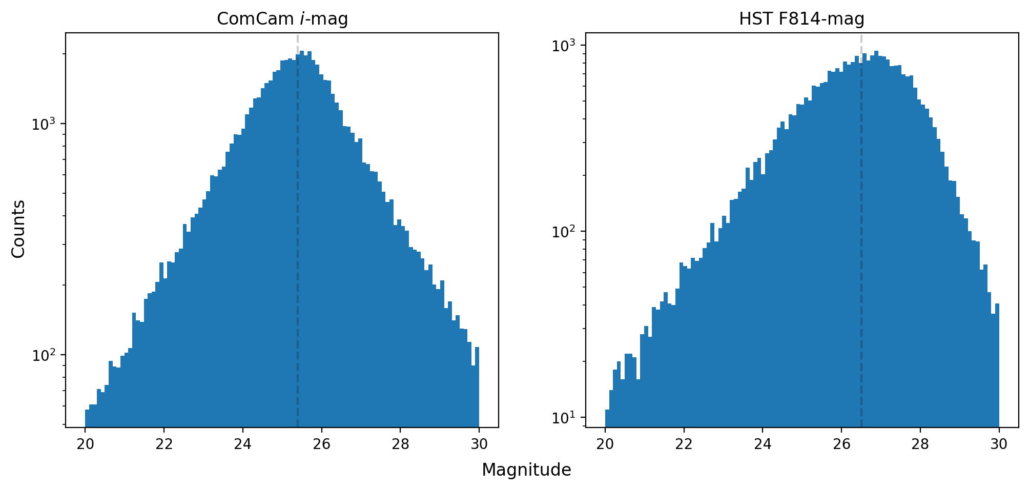
Fig. 7 Log scale histogram of i-magnitude distribution for LSSTComCam and F814W-magnitude for HST. The dashed lines are the approximate completeness limits of 25.4 and 26.5 respectively.#